Mathematical Formulation and Optimization

Spatial Transformer Network and Optimization

Following the settings of previous post (Image Alignment using Brute Force), our objective function for finding the optimal displacement vector is denoted as:

\[dx^*, dy^* = \arg \min_{dx \in X, dy \in Y} L(\text{shift}(A, dx, dy), B)\]

where (X) and (Y) are search spaces, (dx) and (dy) represent the shift in the (x) and (y) directions, (L) is the cost metric, and (A) and (B) are image channels.

Instead of exhaustively searching for the optimal displacement ((dx, dy)) to align the images, we can use a mathematical operation that shifts the image in a way that can be adjusted and optimized. In this case, we apply Spatial Transformation. This approach allows us to express the image shift as a continuous, differentiable operation, which means we can use gradient descent for optimization.

For cost metric, we use Means Squared Error (MSE) and Normalized Correlation Coefficient (NCC).

Affine Transformation for Shifting

The affine transformation matrix for translation can be defined as:

\[\theta = \begin{bmatrix} 1 & 0 & dx \\ 0 & 1 & dy \end{bmatrix}\]

Since we are only performing translation (without scaling, rotation, or shearing), the only trainable parameters in the matrix are (dx) and (dy). This affine transformation matrix is used to generate a grid of coordinates for the shifted version of the input image (A).

Thus, the transformation of a point ((x, y)) using this affine transformation matrix is represented as:

\[T_{\theta} = \begin{bmatrix} 1 & 0 & dx \\ 0 & 1 & dy \end{bmatrix} \begin{bmatrix} x \\ y \\ 1 \end{bmatrix}\]

Optimization Using Gradient Descent

To optimize the image alignment, we minimize a given loss function (L) with respect to the displacement parameters (dx) and (dy). The optimization is performed using gradient descent, which iteratively updates the displacement values in the direction that reduces the loss:

\[dx_{n+1} = dx_n - \alpha \nabla_{dx}L(\text{shift}(A, dx, dy), B)\] \[dy_{n+1} = dy_n - \alpha \nabla_{dy}L(\text{shift}(A, dx, dy), B)\]

where (\alpha) is the learning rate, (n) is the number of iterations, and (\nabla_{dx, dy}L) represents the gradient of the loss function with respect to (dx) and (dy). The image shifting process is performed using bilinear interpolation. This interpolation method provides a more accurate approximation when displacements are not integer values, which helps preserve image quality during the alignment process.

The gradient of (dx) is denoted as:

\[\frac{\partial A^*[x_i', y_i']}{\partial x_i} = \sum_{n=1}^{H} \sum_{m=1}^{W} A[n, m] \, \max(0, 1 - |y_i - n|) \cdot \begin{cases} 0 & \text{if } |m - x_i| \geq 1 \\ 1 & \text{if } m \geq x_i \\ -1 & \text{if } m \leq x_i \end{cases}\]

The gradient of (dy) is denoted as:

\[\frac{\partial A^*[x_i', y_i']}{\partial y_i} = \sum_{n=1}^{H} \sum_{m=1}^{W} A[n, m] \, \max(0, 1 - |x_i - m|) \cdot \begin{cases} 0 & \text{if } |n - y_i| \geq 1 \\ 1 & \text{if } n \geq y_i \\ -1 & \text{if } n \leq y_i \end{cases}\]

where (A^*) is the transformed image (A), shifted by (dx) and (dy), (H) and (W) are the height and width of the image, respectively. This process is repeated for (n) iterations.

Description of Implementation

Learning Rate

Experiments were conducted using three different learning rates: 0.1, 0.01, and 0.001, while keeping the number of optimization steps fixed at 30 for all trials. Among these, the learning rate of 0.001 produced the best overall alignment results. Both the learning rates of 0.01 and 0.001 demonstrated comparable performance in terms of alignment quality, but the 0.001 learning rate provided better alignment than 0.01.

However, When the learning rate was set to 0.1, the performance of the alignment process was significantly poorer. This high learning rate led to suboptimal alignments, suggesting that the updates were too large, causing the optimization to overshoot the optimal solution.

In terms of computational speed, execution times across the different learning rate settings did not show notable differences, suggesting that the learning rate had little impact on the computational efficiency of the alignment process.

Number of Steps

Experiments were conducted using two different steps: 30 and 100, with learning rates of 0.01 and 0.001. For the learning rate of 0.001, the alignment quality remained consistent between 30 and 100 steps, indicating that increasing the number of steps did not yield improvement.

However, with a learning rate of 0.01, there were some alignment quality differences between step sizes 30 and 100.

A significant difference was observed in the execution time between the two step counts. For both the MSE and NCC alignment metrics, the execution time per image was between 0.3 and 0.4 seconds when the step count was set to 30. However, when the step count was increased to 100, the execution time exceeded 1 second per image. This shows that although the alignment quality didn’t improve much with more steps, the computational time increased significantly as the step count increased.

Colorized Outputs

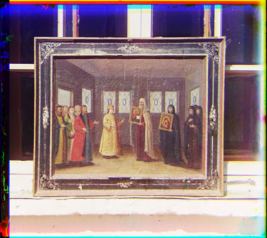
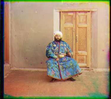
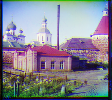
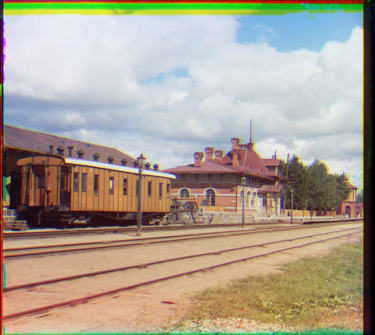
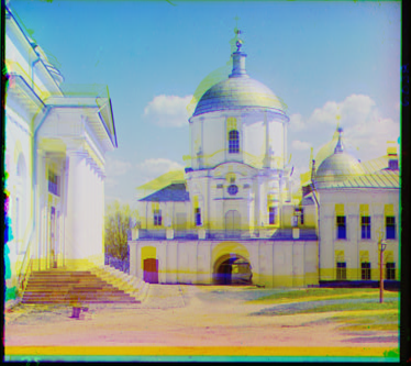
The results are aligned using NCC metric.

Check out the code here!